A Multinomial Naive Bayes classifier trained on a few thousand SMS messages can hit an F1-score that looks production-ready in under a minute. That speed is precisely what makes it a useful teaching model and precisely what makes it a dangerous one to trust without scrutiny. Spam filtering was one of the first domains where adversarial machine learning was studied seriously, with researchers at the 2004 MIT Spam Conference demonstrating that one ML filter could learn to defeat another by automatically selecting which words to inject into a message. If you are going to build a classifier, you need to understand how it learns, how it breaks, and how an attacker sees the gap between the two.

This entry picks up from our earlier work on data preprocessing and feature extraction. We have clean, stemmed text and a CountVectorizer ready to produce numerical features. Now we train, tune, evaluate, and persist a working spam detection model, and we examine what the results actually tell us about robustness.

Building the pipeline

Scikit-learn’s Pipeline object chains the vectorisation and classification steps into a single callable unit. The convenience matters less than the consistency. It ensures that the same transformation is applied identically during training and inference, which eliminates a common source of silent bugs where the vectoriser is fitted on different data or with different parameters at prediction time.

from sklearn.model_selection import train_test_split, GridSearchCV
from sklearn.naive_bayes import MultinomialNB
from sklearn.pipeline import Pipeline

# Build the pipeline by combining vectorisation and classification
pipeline = Pipeline([
    ("vectorizer", vectorizer),
    ("classifier", MultinomialNB())
])

The pipeline takes two named steps. The first is the CountVectorizer instance we built in the previous entry, which converts preprocessed text into a sparse matrix of token counts. The second is a MultinomialNB classifier, which applies Bayes’ theorem under the assumption that features (word counts) follow a multinomial distribution. That assumption is a simplification, words in natural language are not statistically independent, but in practice it works surprisingly well for text classification because the conditional probability estimates remain useful even when the independence assumption is violated.

Hyperparameter tuning with GridSearchCV

A classifier with default parameters is a baseline, not a finished model. GridSearchCV automates the search for better configurations by evaluating every combination of specified parameter values against k-fold cross-validation, then selecting the combination that scores highest on a chosen metric.

For MultinomialNB, the parameter worth tuning is alpha, the Laplace smoothing factor. This value controls what happens when the classifier encounters a word during prediction that appeared in one class but not the other during training. Without smoothing (alpha=0), that word would produce a zero probability, which would dominate the entire classification regardless of every other word in the message. Smoothing adds a small pseudo-count to every feature, preventing any single absent word from collapsing the prediction. Too much smoothing, however, flattens the probability distributions and washes out the signal that distinguishes spam from ham.

# Define the parameter grid for hyperparameter tuning
param_grid = {
    "classifier__alpha": [0.01, 0.1, 0.15, 0.2, 0.25, 0.5, 0.75, 1.0]
}

# Perform the grid search with 5-fold cross-validation and F1-score as metric
grid_search = GridSearchCV(
    pipeline,
    param_grid,
    cv=5,
    scoring="f1"
)

# Fit the grid search on the full dataset
grid_search.fit(df["message"], y)

# Extract the best model identified by the grid search
best_model = grid_search.best_estimator_
print("Best model parameters:", grid_search.best_params_)

We score on F1 rather than accuracy for a specific reason. In a typical SMS dataset, spam accounts for roughly 13 percent of messages. A classifier that labels everything as ham would achieve 87 percent accuracy while catching zero spam. F1 balances precision (of the messages flagged as spam, how many actually were) and recall (of all the actual spam, how much did the classifier catch), which makes it a far more honest metric for imbalanced classes.

The five-fold cross-validation means the dataset is split into five parts, and the model is trained on four parts and tested on the remaining one, rotating through all five. This gives a more reliable estimate of performance than a single train-test split, which can be skewed by an unlucky partition.

Evaluating on unseen messages

The confusion matrix from our tuned model tells a clean story: 889 true negatives, 140 true positives, 5 false positives, and 0 false negatives.

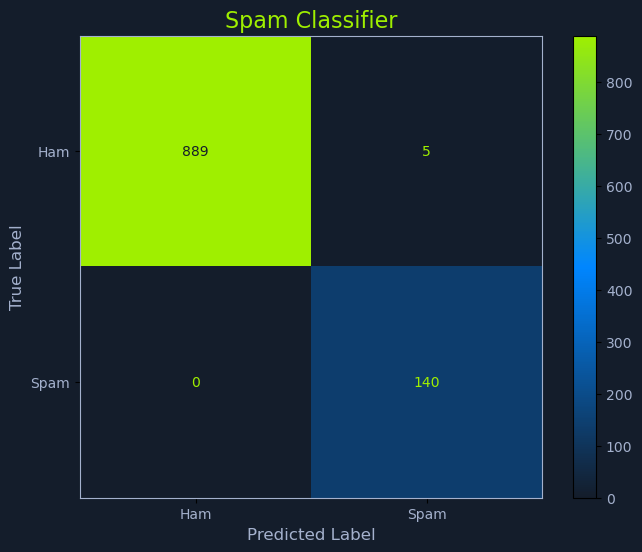
Those numbers look excellent, and that is exactly the moment to be suspicious. Zero false negatives means the classifier caught every spam message in the test set, but the test set was drawn from the same distribution as the training data. Real-world spam does not hold still. Spammers adapt their language, inject legitimate-sounding words, and mutate their templates specifically to evade classifiers like this one.

To get a better sense of how the model behaves on messages it has never seen, we can feed it a small batch of hand-crafted examples that reflect the kinds of messages a deployed classifier would encounter.

# Example SMS messages for evaluation
new_messages = [
    "Congratulations! You've won a $1000 Walmart gift card. Go to http://bit.ly/1234 to claim now.",
    "Hey, are we still meeting up for lunch today?",
    "Urgent! Your account has been compromised. Verify your details here: www.fakebank.com/verify",
    "Reminder: Your appointment is scheduled for tomorrow at 10am.",
    "FREE entry in a weekly competition to win an iPad. Just text WIN to 80085 now!",
]

Before these messages can enter the model, they must pass through the same preprocessing pipeline used during training. This is a non-negotiable requirement. If the training data was lowercased, stripped of non-alphabetic characters, tokenised, stop-word filtered, and stemmed, then the evaluation data must be too. A mismatch here does not produce an error; it produces silently wrong predictions, which is worse.

import numpy as np
import re

def preprocess_message(message):
    message = message.lower()
    message = re.sub(r"[^a-z\s$!]", "", message)
    tokens = word_tokenize(message)
    tokens = [word for word in tokens if word not in stop_words]
    tokens = [stemmer.stem(word) for word in tokens]
    return " ".join(tokens)

# Preprocess the evaluation messages
processed_messages = [preprocess_message(msg) for msg in new_messages]

With the messages preprocessed, we extract the vectoriser and classifier from the pipeline separately. This is useful when you want to inspect intermediate representations or debug prediction behaviour, because it lets you see exactly what the vectoriser produced before the classifier made its decision.

# Transform preprocessed messages into feature vectors
X_new = best_model.named_steps["vectorizer"].transform(processed_messages)

# Predict with the trained classifier
predictions = best_model.named_steps["classifier"].predict(X_new)
prediction_probabilities = best_model.named_steps["classifier"].predict_proba(X_new)

The output gives us both a binary label and the probability estimates behind it, which is where things get interesting from a red team perspective.

for i, msg in enumerate(new_messages):
    prediction = "Spam" if predictions[i] == 1 else "Not-Spam"
    spam_probability = prediction_probabilities[i][1]
    ham_probability = prediction_probabilities[i][0]

    print(f"Message: {msg}")
    print(f"Prediction: {prediction}")
    print(f"Spam Probability: {spam_probability:.2f}")
    print(f"Not-Spam Probability: {ham_probability:.2f}")
    print("-" * 50)

Message: Congratulations! You've won a $1000 Walmart gift card. Go to http://bit.ly/1234 to claim now.
Prediction: Spam
Spam Probability: 1.00
Not-Spam Probability: 0.00
--------------------------------------------------
Message: Hey, are we still meeting up for lunch today?
Prediction: Not-Spam
Spam Probability: 0.00
Not-Spam Probability: 1.00
--------------------------------------------------
Message: Urgent! Your account has been compromised. Verify your details here: www.fakebank.com/verify
Prediction: Spam
Spam Probability: 0.94
Not-Spam Probability: 0.06
--------------------------------------------------
Message: Reminder: Your appointment is scheduled for tomorrow at 10am.
Prediction: Not-Spam
Spam Probability: 0.00
Not-Spam Probability: 1.00
--------------------------------------------------
Message: FREE entry in a weekly competition to win an iPad. Just text WIN to 80085 now!
Prediction: Spam
Spam Probability: 1.00
Not-Spam Probability: 0.00
--------------------------------------------------

The classifier correctly identifies all five messages, and the probability estimates show high confidence. But notice the third message, the phishing attempt, sits at 0.94 rather than 1.00. That six percent uncertainty is worth paying attention to. The message uses language (“account”, “verify”, “details”) that legitimately appears in ham messages from banks and service providers, which pulls the probability toward ham even though the overall message is clearly malicious. An attacker who understood this could add more legitimate-sounding words to push that probability below the classification threshold.

Saving the model with joblib

Once a model is trained, tuned, and evaluated, retraining it from scratch every time the application starts is wasteful. joblib serialises the entire pipeline, including the fitted vectoriser’s vocabulary and the classifier’s learned probability tables, into a binary file that can be reloaded instantly.

import joblib

# Save the trained model to a file for future use
model_filename = 'spam_detection_model.joblib'
joblib.dump(best_model, model_filename)
print(f"Model saved to {model_filename}")

Serialisation here means converting the in-memory Python objects into a binary format that preserves their complete state. When joblib saves a scikit-learn pipeline, it captures the vectoriser’s learned vocabulary mapping, the classifier’s conditional probability tables, the smoothing parameter, and every other fitted attribute. joblib is preferred over Python’s built-in pickle for scikit-learn models because it handles large NumPy arrays more efficiently, using memory mapping and compression to reduce file size and load time.

Loading the model back is a single call, and the restored object is immediately ready to predict.

# Load the saved model
loaded_model = joblib.load(model_filename)

# Preprocess new messages before prediction
new_data_processed = [preprocess_message(msg) for msg in new_messages]

# Make predictions on the preprocessed data
predictions = loaded_model.predict(new_data_processed)

There is one important caveat. The serialised model captures the vectoriser and classifier, but it does not capture the preprocessing function. If you change preprocess_message after saving the model (perhaps by adding a new stop word or switching from Porter to Snowball stemming), the loaded model will still expect text in the old format. In production, the preprocessing logic either needs to be versioned alongside the model or wrapped into a custom scikit-learn transformer and included in the pipeline itself.

What the red team sees

This classifier works. It catches obvious spam with high confidence, correctly passes legitimate messages, and even handles the ambiguous phishing case with reasonable probability estimates. But from an adversarial perspective, the model has several properties worth noting.

Multinomial Naive Bayes is a linear classifier. Its decision boundary is a hyperplane in the feature space, which means an attacker who can estimate which words carry high ham probability can craft messages that cross that boundary by injecting a handful of carefully chosen tokens. This is not theoretical. Researchers demonstrated exactly this technique against SpamBayes in 2006, showing that an attacker with access to just one percent of the training data could render the filter useless.

The predict_proba output we examined earlier is itself a signal. If an attacker can query the model (and in many deployed systems, the spam/not-spam decision is visible to the sender through delivery receipts or bounce messages), they can probe the boundary iteratively, adjusting their message until it slips through.

The model also has no concept of message structure, sender reputation, or temporal patterns. It sees a bag of words and nothing else. A message that says “free win prize claim now” and a message that embeds those same words inside an otherwise legitimate paragraph produce different feature vectors, but the classifier’s only defence is the relative counts.

These are not reasons to discard Naive Bayes. They are reasons to understand what it is actually doing, so that when we start examining adversarial attacks in later entries, we have a concrete model to attack rather than an abstract concept to theorise about.

The spam classifier you just built is your first target.